Of the importance of normalisation
Of the importance of normalisation#
This SOM implementation will initialise by default the weight vectors or the neurons to random values using a Gaussian distribution with zero mean and unity standard deviation. This means that the weight vectors will have values mostly between -1 and 1.
If the train and test data have values which are not normalised, that is with zero mean and a standard deviation of one, there is a chance that the fitting procedure will, in the best case, yield unsatisfactory resulst, and in the worst case, completely fail.
To solve this issue, it can be beneficial to normalise the data beforehand.
Note
The normalisation of the data will will affect the fitting procedure in various ways. Weight vectors initialised far from the data will:
not train in a similar fashion as if they were intialised close to the data
require more steps to converge
potentially not converge enough since the convergence of the neurons is reduced as the training phase proceeds
We will illustrate the importance of normalisation in an example. To do so, we will generate clusters of data with random \((x, y)\) coordinates using a normal distribution:
Code
import numpy        as     np
from   numpy.random import default_rng
rng = default_rng()

# Random x coordinates
x = []
x = np.concatenate((x, rng.normal(loc=0, scale=1, size=100)))
x = np.concatenate((x, rng.normal(loc=10, scale=1, size=100)))
x = np.concatenate((x, rng.normal(loc=-3, scale=1, size=100)))
x = np.concatenate((x, rng.normal(loc=16, scale=1, size=100)))
x = np.concatenate((x, rng.normal(loc=-6, scale=1, size=100)))
x = np.concatenate((x, rng.normal(loc=-10, scale=1, size=100)))
x = np.concatenate((x, rng.normal(loc=13, scale=1, size=100)))
x = np.concatenate((x, rng.normal(loc=-6, scale=1, size=100)))

# Random y coordinates
y = []
y = np.concatenate((y, rng.normal(loc=20, scale=1, size=100)))
y = np.concatenate((y, rng.normal(loc=-10, scale=1, size=100)))
y = np.concatenate((y, rng.normal(loc=-10, scale=1, size=100)))
y = np.concatenate((y, rng.normal(loc=7, scale=1, size=100)))
y = np.concatenate((y, rng.normal(loc=-10, scale=1, size=100)))
y = np.concatenate((y, rng.normal(loc=0, scale=1, size=100)))
y = np.concatenate((y, rng.normal(loc=-16, scale=1, size=100)))
y = np.concatenate((y, rng.normal(loc=-8, scale=1, size=100)))

# Combine coordinates to have an array of the correct shape for the SOM to train onto
data = np.array([x, y]).T

print(data.shape)
Results
(800, 2)
To begin with, we will not normalise the data. For illustration purposes, we will set the seed of the SOM weight initialisation so that we know the initial values of the SOM. However, we will not disable shuffling because of the way we built our dataset. Indeed, we built the clusters one after the other. This means that when training the SOM without shuffling, the neuron closest to the first cluster will be trained until the cluster has been exhausted, then the neuron closest to the second cluster will be trained and so on. In the end, the training will be biased by the fact that neurons are not trained at the same frequency.
Let us train the SOM onto this dataset:
from SOMptimised import SOM, LinearLearningStrategy, ConstantRadiusStrategy, euclidianMetric

lr     = LinearLearningStrategy(lr=1)      # Learning rate strategy
sigma  = ConstantRadiusStrategy(sigma=0.1) # Neighbourhood radius strategy
metric = euclidianMetric                   # Metric used to compute BMUs
nf     = data.shape[1]                     # Number of features
som    = SOM(m=2, n=4, dim=nf, lr=lr, sigma=sigma, metric=metric, max_iter=1e4, random_state=0)
som.fit(data, epochs=3, shuffle=True)

# Prediction for the train dataset
pred   = som.train_bmus_
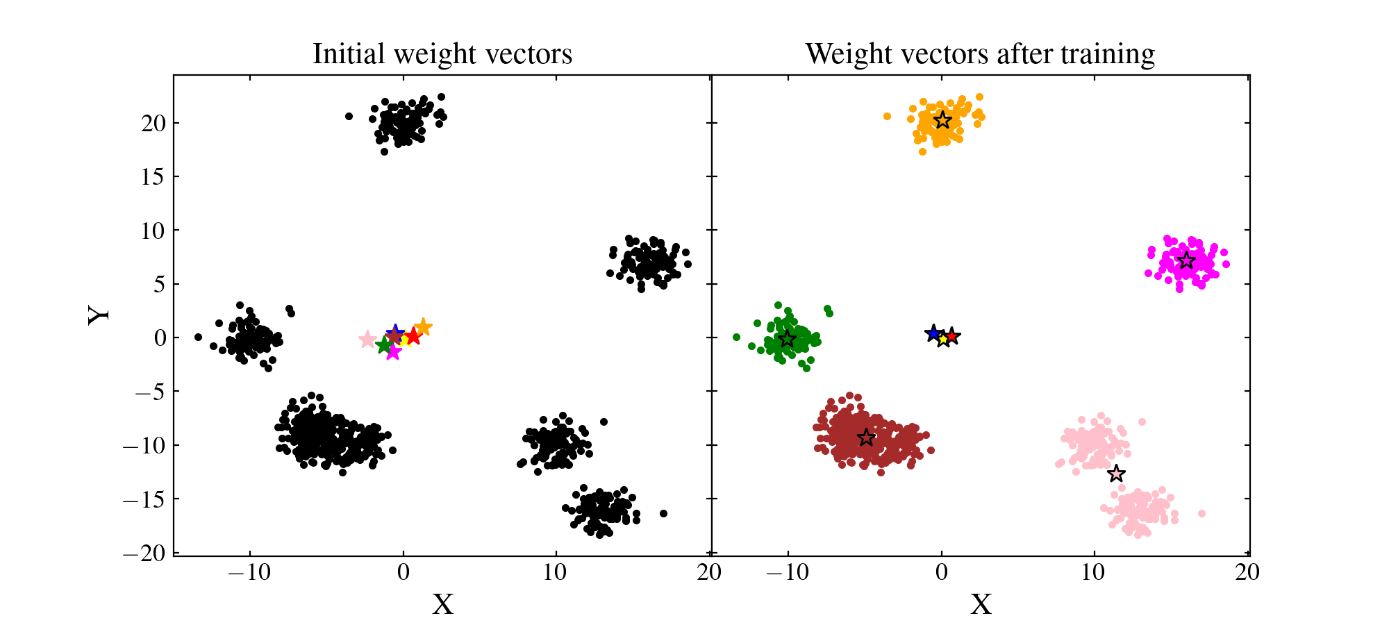
Let us see how the SOM performed. We will plot on the left figure the data with black points and the initial random weights values as coloured stars. On the right figure, we will plot the trained SOM weight values as coloured stars and the data as coloured points which matches that of their BMU:
import matplotlib.pyplot   as     plt
from   matplotlib          import rc
from   matplotlib.gridspec import GridSpec

rc('font', **{'family': 'serif', 'serif': ['Times']})
rc('text', usetex=True)

f  = plt.figure(figsize=(10, 4.5))
gs = GridSpec(1, 2, wspace=0, hspace=0)

#####################
#     Left plot     #
#####################

ax1 = f.add_subplot(gs[0])

ax1.yaxis.set_ticks_position('both')
ax1.xaxis.set_ticks_position('both')
ax1.tick_params(axis='x', which='both', direction='in', labelsize=13, length=3)
ax1.tick_params(axis='y', which='both', direction='in', labelsize=13, length=3)
ax1.set_ylabel('Y', size=16)
ax1.set_xlabel('X', size=16)
ax1.set_title('Initial weight vectors', size=16)

# We recompute the initial weight values (this is possible because we set the seed of the random generator)
rng     = np.random.default_rng(0)
weights = rng.normal(size=(2*4, nf))

colors  = ['yellow', 'r', 'b', 'orange', 'magenta', 'brown', 'pink', 'g']

# Plot neurons
for xx, yy, c in zip(weights[:, 0], weights[:, 1], colors):
   ax1.plot(xx, yy, marker='*', color=c, linestyle='none', markersize=10)

# Plot train data
ax1.plot(x, y, 'k.', linestyle='none')

######################
#     Right plot     #
######################

ax2 = f.add_subplot(gs[1])

ax2.yaxis.set_ticks_position('both')
ax2.xaxis.set_ticks_position('both')
ax2.tick_params(axis='x', which='both', direction='in', labelsize=13, length=3)
ax2.tick_params(axis='y', which='both', direction='in', labelsize=13, length=3)
ax2.set_xlabel('X', size=16)
ax2.set_title('Weight vectors after training', size=16)
ax2.set_yticklabels([])

for idx, xx, yy, c in zip(range(som.weights.shape[0]), som.weights[:, 0], som.weights[:, 1], colors):

   # Find data which have this neuron as BMU
   data_idx = data[pred == idx]

   ax2.plot(data_idx[:, 0], data_idx[:, 1], color=c, marker='.', linestyle='none')
   ax2.plot(xx, yy, marker='*', color=c, linestyle='none', markersize=10, mec='k')

plt.show()
(Source code, png, hires.png, pdf)

We see that the result if far from being optimal. Even if some clusters are recovered by the SOM, some neurons are far from where they should ideally converge. Besides, even those which are near clusters are somewhat offset from their ideal position. The reason for this effect is that the data have not been normalised. A neuron which is initialised at a privileged position with respect to some cluster will have more chance to being trained and pulled onto that cluster, making other neurons less likely to be trained efficiently.
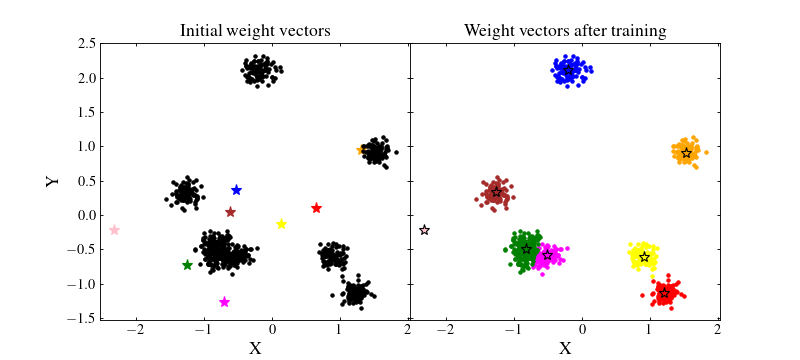
To circumvent this problem we can normalise the data by removing the mean value and dividing by their standard deviation for each feature. This way, the majority of the data should be located in the range \([-1, 1]\), near the random initial positions of the SOM wieght vectors:
# Print mean and std before normalisation
print(f'Mean along x and y axes before normalisation: {np.nanmean(data, axis=0)}')
print(f'Standard deviation along x and y axes before normalisation: {np.nanstd(data, axis=0)}')

# Normalise each feature
new_data = (data - np.nanmean(data, axis=0))/np.nanstd(data, axis=0)

# Print mean and std after normalisation
print(f'Mean along x and y axes after normalisation: {np.nanmean(data, axis=0)}')
print(f'Standard deviation along x and y axes after normalisation: {np.nanstd(data, axis=0)}')
Results
Mean before normalisation: [ 1.77566182 -3.39528932]
Standard deviation before normalisation: [ 9.25872052 11.11128508]
Mean after normalisation: [0.00000000e+00 3.55271368e-17]
Standard deviation after normalisation: [1. 1.]
Now, we can train again the SOM and see whether the normalisation changed anything
som    = SOM(m=2, n=4, dim=nf, lr=lr, sigma=sigma, metric=metric, max_iter=1e4, random_state=0)
som.fit(data_norm, epochs=3, shuffle=True)

# Prediction for the train dataset
pred   = som.train_bmus_

# Plotting
rc('font', **{'family': 'serif', 'serif': ['Times']})
rc('text', usetex=True)

f  = plt.figure(figsize=(10, 4.5))
gs = GridSpec(1, 2, wspace=0, hspace=0)

#####################
#     Left plot     #
#####################

ax1 = f.add_subplot(gs[0])

ax1.yaxis.set_ticks_position('both')
ax1.xaxis.set_ticks_position('both')
ax1.tick_params(axis='x', which='both', direction='in', labelsize=13, length=3)
ax1.tick_params(axis='y', which='both', direction='in', labelsize=13, length=3)
ax1.set_ylabel('Y', size=16)
ax1.set_xlabel('X', size=16)
ax1.set_title('Initial weight vectors', size=16)

# We recompute the initial weight values (this is possible because we set the seed of the random generator)
rng     = np.random.default_rng(0)
weights = rng.normal(size=(2*4, nf))

colors  = ['yellow', 'r', 'b', 'orange', 'magenta', 'brown', 'pink', 'g']

# Plot neurons
for xx, yy, c in zip(weights[:, 0], weights[:, 1], colors):
   ax1.plot(xx, yy, marker='*', color=c, linestyle='none', markersize=10)

# Plot train data
ax1.plot(data_norm[:, 0], data_norm[:, 1], 'k.', linestyle='none')

######################
#     Right plot     #
######################

ax2 = f.add_subplot(gs[1])

ax2.yaxis.set_ticks_position('both')
ax2.xaxis.set_ticks_position('both')
ax2.tick_params(axis='x', which='both', direction='in', labelsize=13, length=3)
ax2.tick_params(axis='y', which='both', direction='in', labelsize=13, length=3)
ax2.set_xlabel('X', size=16)
ax2.set_title('Weight vectors after training', size=16)
ax2.set_yticklabels([])

for idx, xx, yy, c in zip(range(som.weights.shape[0]), som.weights[:, 0], som.weights[:, 1], colors):

   # Find data which have this neuron as BMU
   data_idx = data_norm[pred == idx]

   ax2.plot(data_idx[:, 0], data_idx[:, 1], color=c, marker='.', linestyle='none')
   ax2.plot(xx, yy, marker='*', color=c, linestyle='none', markersize=10, mec='k')

plt.show()
(Source code, png, hires.png, pdf)

Important
Normalisation is not always the best option. It all comes down to the metric used.
For instance, with the chi2CigaleMetric() metric, data should not be normalised. Instead, to have an optimal SOM, one should denormalise the SOM weight vectors using unnormalise_weights=True when calling the fit() method.
See the documentation for the metric you use for more information.