Train the SOM to predict the iris class
Train the SOM to predict the iris class#
We will use the SOM to predict the iris class of the test set. We can see by eye than there must be something like three different classes in the iris dataset so we will use a small SOM of dimensions (1, 3) so that each neuron will predict a given class.
First let us create a SOM object with the right properties
from SOMptimised import SOM, LinearLearningStrategy, ConstantRadiusStrategy, euclidianMetric

lr     = LinearLearningStrategy(lr=1)      # Learning rate strategy
sigma  = ConstantRadiusStrategy(sigma=0.8) # Neighbourhood radius strategy
metric = euclidianMetric                   # Metric used to compute BMUs
nf     = data_train.shape[1]               # Number of features
som    = SOM(m=1, n=3, dim=nf, lr=lr, sigma=sigma, max_iter=1e4, random_state=None)
The various parameters appearing when creating the SOM object are:
m and n: the vertical and horizontal dimensions of the SOM, respectively
dim: the number of features in the data
lr: the learning rate strategy. Any strategy can be used as long as it inherits from
LearningStrategy. Here, we will use a learning rate which linearly decreases with learning steps.sigma: the neighboorhood radius strategy. Any strategy can be used as long as it inherits from
NeighbourhoodStrategy. Here, we will use a constant neighbourhood radius. The larger the radius the more aggressive the SOM.metric: the metric used to compute the distance between the SOM neurons and the training data, and between the test data and the neurons. Any metric can be used. See the metric documentation for the available metrics and how to implement new ones.
max_iter: the maximum number of iterations. The learning will continue until the number of iterations becomes equal to
min(max_iter, len(data)*epochs)whereepochsis the number of epochs used during the fit.random_state: if not
None, must be an integer. This defines the random_state used to generate random initial values for the weights before starting the fit. Setting a value can be useful for debugging.
Training the som is quite straightforward. This can be done the following way
som.fit(data_train, epochs=1, shuffle=True, n_jobs=1)
The parameter shuffle means the train data will be shuffled at each new epoch. The parameter n_jobs sets the number of threads used on the computer to compute the BMUs at the end of the training.
Note
Using the maximum number of threads is not necessarily optimal, unless the train data and/or the neurons are very numerous.
We can now predict the class for the test set
pred_test = som.predict(data_test)
print(pred_test)
Results
[0 0 0 0 0]
Similarly we can extract the predictions the SOM made on the training dataset
pred_train = som.train_bmus_
print(pred_train)
Results
[0 0 0 0 0 0 0 0 0 0 0 0 0 0 0 0 0 0 0 0 0 0 0 0 0 0 0 0 0 0 0 0 0 0 0 0 0
 0 0 0 0 0 0 0 0 0 0 0 0 0 2 2 2 1 2 1 2 1 2 1 1 1 1 2 1 2 1 1 2 1 2 1 2 2
 2 2 2 2 2 1 1 1 1 2 1 2 2 2 1 1 1 2 1 1 1 1 1 1 1 1 2 2 2 2 2 2 1 2 2 2 2
 2 2 2 2 2 2 2 2 2 2 2 2 2 2 2 2 2 2 2 2 2 2 2 2 2 2 2 2 2 2 2 2 2 2]
The SOM does not directly give us the predicted class but rather the closest neuron in the SOM for each data point. Because there are only three neurons, we can neverthelss associate them to a class.
Let us plot the training (small points) and test (large points) datasets colour coded by their best-matching unit which will act as a class
import matplotlib.pyplot   as     plt
from   matplotlib.colors   import TwoSlopeNorm
from   matplotlib.gridspec import GridSpec
from   matplotlib          import rc
import matplotlib           as    mpl

norm = TwoSlopeNorm(1, vmin=0, vmax=2)

rc('font', **{'family': 'serif', 'serif': ['Times']})
rc('text', usetex=True)
mpl.rcParams['text.latex.preamble'] = r'\usepackage{newtxmath}'

f   = plt.figure(figsize=(10, 4.5))
gs  = GridSpec(1, 2, wspace=0)
ax1 = f.add_subplot(gs[0])
ax2 = f.add_subplot(gs[1])

for ax in [ax1, ax2]:
    ax.yaxis.set_ticks_position('both')
    ax.xaxis.set_ticks_position('both')
    ax.tick_params(axis='x', which='both', direction='in', labelsize=13, length=3)
    ax.tick_params(axis='y', which='both', direction='in', labelsize=13, length=3)
    ax.set_xlabel('Petal width (cm)', size=16)

ax1.scatter(data_train[:, 1], data_train[:, 0], c=pred_train, cmap='bwr', ec='k', norm=norm, marker='o', s=30)
ax1.scatter(data_test[:, 1],  data_test[:, 0],  c=pred_test,  cmap='bwr', ec='k', marker='o', norm=norm, s=60)
ax1.set_ylabel('Petal length (cm)', size=16)

target                              = target.to_numpy()
target[target == 'Iris-setosa']     = 0
target[target == 'Iris-versicolor'] = 1
target[target == 'Iris-virginica']  = 2

ax2.scatter(data_train[:, 1], data_train[:, 0], c=target[:-10], cmap='bwr', ec='k', norm=norm, marker='o', s=30)
ax2.scatter(data_test[:, 1],  data_test[:, 0],  c=target[-10:],  cmap='bwr', ec='k', marker='o', norm=norm, s=60)
ax2.set_yticks([0.2])
ax2.set_yticklabels([])

ax1.set_title('SOM clustering', size=18)
ax2.set_title('IRIS dataset', size=18)

plt.show()
(Source code, png, hires.png, pdf)
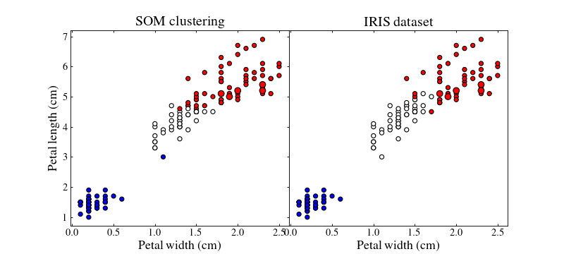
By playing with the different parameters of the SOM and the different strategies we can achieve better or worse results.
Note
Colours do not match between subfigures, they are just here to show clustering.