Tutorial/Example
Contents
Tutorial/Example#
Important
This example requires pandas to be installed. This can be done the following way with pip
pip install pandas
or with conda
conda install pandas
Preparing the data#
This SOM implementation requires the data to be given as a 2-dimensional numpy array where the first dimension corresponds to the observations or data points that you have and the second dimension corresponds to the features for each observation.
Let us run the SOM on the iris dataset. To do so we will use pandas to load the dataset contained in the csv file
Code
import pandas

table = pandas.read_csv('examples/iris_dataset/iris_dataset.csv')
print(table.head(), end='\n\n')
print(table.info())
Results
   sepal length (cm)  sepal width (cm)  petal length (cm)  petal width (cm)       target
0                5.1               3.5                1.4               0.2  Iris-setosa
1                4.9               3.0                1.4               0.2  Iris-setosa
2                4.7               3.2                1.3               0.2  Iris-setosa
3                4.6               3.1                1.5               0.2  Iris-setosa
4                5.0               3.6                1.4               0.2  Iris-setosa

<class 'pandas.core.frame.DataFrame'>
RangeIndex: 150 entries, 0 to 149
Data columns (total 5 columns):
 #   Column             Non-Null Count  Dtype
---  ------             --------------  -----
 0   sepal length (cm)  150 non-null    float64
 1   sepal width (cm)   150 non-null    float64
 2   petal length (cm)  150 non-null    float64
 3   petal width (cm)   150 non-null    float64
 4   target             150 non-null    object
dtypes: float64(4), object(1)
memory usage: 6.0+ KB
None
Each line represents an observation and in this case we have 4 features: sepal length, sepal width, petal length and petal width. Let us train the SOM on three features
table  = table[['petal length (cm)', 'petal width (cm)', 'sepal length (cm)']]
target = table['target']
swidth = table['sepal width (cm)']
print(table.info())
Results
<class 'pandas.core.frame.DataFrame'>
RangeIndex: 150 entries, 0 to 149
Data columns (total 3 columns):
 #   Column             Non-Null Count  Dtype
---  ------             --------------  -----
 0   petal length (cm)  150 non-null    float64
 1   petal width (cm)   150 non-null    float64
 2   sepal length (cm)  150 non-null    float64
dtypes: float64(3)
memory usage: 3.6 KB
None
where we have also extracted the target class for each observation to compare at the end and the sepal width to predict for the next section. We convert the data into a numpy array since this is the required format for the SOM to run and we check it has the correct shape (150, 3)
data  = table.to_numpy()
print(data.shape)
print(data[:5])
Results
(150, 3)
[[1.4 0.2 5.1]
 [1.4 0.2 4.9]
 [1.3 0.2 4.7]
 [1.5 0.2 4.6]
 [1.4 0.2 5. ]]
Finally, let us keep the last five observations apart to test the SOM
data_train = data[:-5]
data_test  = data[-5:]
print(len(data_train), len(data_test))
Results
145 5
Train the SOM to predict the iris class#
We will use the SOM to predict the iris class of the test set. We can see by eye than there must be something like three different classes in the iris dataset so we will use a small SOM of dimensions (1, 3) so that each neuron will predict a given class.
First let us create a SOM object with the right properties
from SOMptimised import SOM, LinearLearningStrategy, ConstantRadiusStrategy, euclidianMetric

lr     = LinearLearningStrategy(lr=1)      # Learning rate strategy
sigma  = ConstantRadiusStrategy(sigma=0.8) # Neighbourhood radius strategy
metric = euclidianMetric                   # Metric used to compute BMUs
nf     = data_train.shape[1]               # Number of features
som    = SOM(m=1, n=3, dim=nf, lr=lr, sigma=sigma, max_iter=1e4, random_state=None)
The various parameters appearing when creating the SOM object are:
m and n: the vertical and horizontal dimensions of the SOM, respectively
dim: the number of features in the data
lr: the learning rate strategy. Any strategy can be used as long as it inherits from
LearningStrategy. Here, we will use a learning rate which linearly decreases with learning steps.sigma: the neighboorhood radius strategy. Any strategy can be used as long as it inherits from
NeighbourhoodStrategy. Here, we will use a constant neighbourhood radius. The larger the radius the more aggressive the SOM.metric: the metric used to compute the distance between the SOM neurons and the training data, and between the test data and the neurons. Any metric can be used. See the metric documentation for the available metrics and how to implement new ones.
max_iter: the maximum number of iterations. The learning will continue until the number of iterations becomes equal to
min(max_iter, len(data)*epochs)whereepochsis the number of epochs used during the fit.random_state: if not
None, must be an integer. This defines the random_state used to generate random initial values for the weights before starting the fit. Setting a value can be useful for debugging.
Training the som is quite straightforward. This can be done the following way
som.fit(data_train, epochs=1, shuffle=True, n_jobs=1)
The parameter shuffle means the train data will be shuffled at each new epoch. The parameter n_jobs sets the number of threads used on the computer to compute the BMUs at the end of the training.
Note
Using the maximum number of threads is not necessarily optimal, unless the train data and/or the neurons are very numerous.
We can now predict the class for the test set
pred_test = som.predict(data_test)
print(pred_test)
Results
[0 0 0 0 0]
Similarly we can extract the predictions the SOM made on the training dataset
pred_train = som.train_bmus_
print(pred_train)
Results
[2 2 2 2 2 2 2 2 2 2 2 2 2 2 2 2 2 2 2 2 2 2 2 2 2 2 2 2 2 2 2 2 2 2 2 2 2
 2 2 2 2 2 2 2 2 2 2 2 2 2 0 0 0 1 0 1 0 1 0 1 1 1 1 0 1 0 1 1 1 1 0 1 0 1
 1 0 0 0 1 1 1 1 1 0 1 1 0 1 1 1 1 1 1 1 1 1 1 1 2 1 0 0 0 0 0 0 1 0 0 0 0
 0 0 0 0 0 0 0 0 0 0 0 0 0 0 0 0 0 0 0 0 0 0 0 0 0 0 0 0 0 0 0 0 0 0]
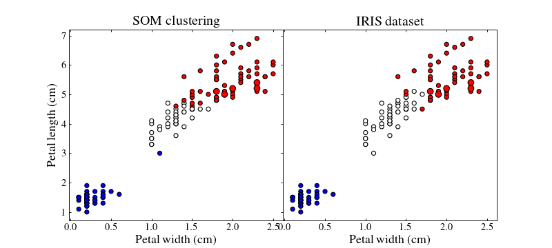
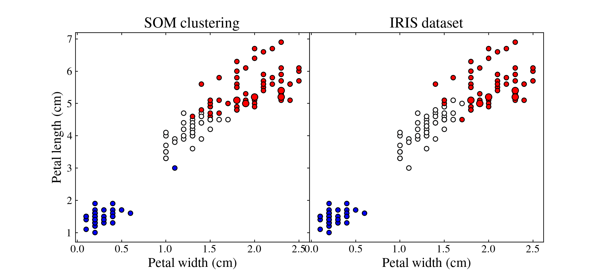
The SOM does not directly give us the predicted class but rather the closest neuron in the SOM for each data point. Because there are only three neurons, we can neverthelss associate them to a class.
Let us plot the training (small points) and test (large points) datasets colour coded by their best-matching unit which will act as a class
import matplotlib.pyplot   as     plt
from   matplotlib.colors   import TwoSlopeNorm
from   matplotlib.gridspec import GridSpec
from   matplotlib          import rc
import matplotlib           as    mpl

norm = TwoSlopeNorm(1, vmin=0, vmax=2)

rc('font', **{'family': 'serif', 'serif': ['Times']})
rc('text', usetex=True)
mpl.rcParams['text.latex.preamble'] = r'\usepackage{newtxmath}'

f   = plt.figure(figsize=(10, 4.5))
gs  = GridSpec(1, 2, wspace=0)
ax1 = f.add_subplot(gs[0])
ax2 = f.add_subplot(gs[1])

for ax in [ax1, ax2]:
    ax.yaxis.set_ticks_position('both')
    ax.xaxis.set_ticks_position('both')
    ax.tick_params(axis='x', which='both', direction='in', labelsize=13, length=3)
    ax.tick_params(axis='y', which='both', direction='in', labelsize=13, length=3)
    ax.set_xlabel('Petal width (cm)', size=16)

ax1.scatter(data_train[:, 1], data_train[:, 0], c=pred_train, cmap='bwr', ec='k', norm=norm, marker='o', s=30)
ax1.scatter(data_test[:, 1],  data_test[:, 0],  c=pred_test,  cmap='bwr', ec='k', marker='o', norm=norm, s=60)
ax1.set_ylabel('Petal length (cm)', size=16)

target                              = target.to_numpy()
target[target == 'Iris-setosa']     = 0
target[target == 'Iris-versicolor'] = 1
target[target == 'Iris-virginica']  = 2

ax2.scatter(data_train[:, 1], data_train[:, 0], c=target[:-10], cmap='bwr', ec='k', norm=norm, marker='o', s=30)
ax2.scatter(data_test[:, 1],  data_test[:, 0],  c=target[-10:],  cmap='bwr', ec='k', marker='o', norm=norm, s=60)
ax2.set_yticks([0.2])
ax2.set_yticklabels([])

ax1.set_title('SOM clustering', size=18)
ax2.set_title('IRIS dataset', size=18)

plt.show()
(Source code, png, hires.png, pdf)

By playing with the different parameters of the SOM and the different strategies we can achieve better or worse results.
Note
Colours do not match between subfigures, they are just here to show clustering.
Predict sepal width#
We can also use the SOM to predict additional features of the test dataset. To do so, we first need to assign new features to the neurons of the SOM.
Let us predict the sepal width of the test dataset using our SOM. To do so we will train a new SOM with more neurons to have finer predictions
import pandas
from   SOMptimised import SOM, LinearLearningStrategy, ConstantRadiusStrategy, euclidianMetric
import numpy       as np

# Extract data
table        = pandas.read_csv('examples/iris_dataset/iris_dataset.csv').sample(frac=1)
swidth       = table['sepal width (cm)'].to_numpy()
data         = table[['petal length (cm)', 'petal width (cm)', 'sepal length (cm)']].to_numpy()

data_train   = data[:-10]
data_test    = data[-10:]
swidth_train = swidth[:-10]
swidth_test  = swidth[-10:]

# Fit SOM
m      = 5
n      = 5
lr     = LinearLearningStrategy(lr=1)      # Learning rate strategy
sigma  = ConstantRadiusStrategy(sigma=0.8) # Neighbourhood radius strategy
metric = euclidianMetric                   # Metric used to compute BMUs
nf     = data_train.shape[1]               # Number of features

som    = SOM(m=m, n=n, dim=nf, lr=lr, sigma=sigma, metric=metric, max_iter=1e4, random_state=None)
som.fit(data_train, epochs=1, shuffle=True, n_jobs=1)

pred_train = som.train_bmus_
pred_test  = som.predict(data_test)
Here we used a \(5 \times 5\) SOM to fit the data. A larger SOM might give more precise results but some neurons might never map to any data point though.
We also extract the sepal width column of the train and test datasets. The sepal width for the test dataset will be used to compare with the predicition from the SOM. That of the train dataset will be used to assign a sepal width for each neuron in the SOM.
To compute a sepal width estimate for each neuron, we can loop through them and find all data points whose best-matching unit is that neuron. The sepal width of the neuron can then be computed as the median value of the sepal width of all these data points
# Compute median sepal width and uncertainty for all neurons
swidth_med = []
swidth_std = []

for i in range(m*n):
    tmp    = swidth_train[pred_train == i]

    swidth_med.append(np.nanmedian(tmp))
    swidth_std.append(np.nanstd(tmp))
In the code above, we also computed an estimate of the uncertainty on the sepal width as the standard deviation. Lets us predict the sepal width of the test set using the SOM
# Predict sepal width for test set
swidth_test_pred     = np.array(swidth_med)[pred_test]
swidth_test_pred_std = np.array(swidth_std)[pred_test]

print('Predicted     Real')
for pred, err, true in zip(swidth_test_pred, swidth_test_pred_std, swidth_test):
    print(f'{pred:.1f} +- {err:.1f}    {true:.1f}')
Results
Predicted     Real
3.0 +- 0.3    2.8
2.7 +- 0.2    2.9
3.0 +- 0.3    3.3
3.1 +- 0.1    3.0
3.0 +- 0.3    2.7
2.9 +- 0.3    3.3
3.0 +- 0.3    3.0
3.5 +- 0.2    3.3
3.0 +- 0.3    3.2
3.5 +- 0.2    3.8
Note
Depending on the parameters of the SOM and the initialisation of the weights, it is not possible to predict a sepal width for all the data points in the test dataset.
Of the importance of normalisation#
This SOM implementation will initialise by default the weight vectors or the neurons to random values using a Gaussian distribution with zero mean and unity standard deviation. This means that the weight vectors will have values mostly between -1 and 1.
If the train and test data have values which are not normalised, that is with zero mean and a standard deviation of one, there is a chance that the fitting procedure will, in the best case, yield unsatisfactory resulst, and in the worst case, completely fail.
To solve this issue, it can be beneficial to normalise the data beforehand.
Note
The normalisation of the data will will affect the fitting procedure in various ways. Weight vectors initialised far from the data will:
not train in a similar fashion as if they were intialised close to the data
require more steps to converge
potentially not converge enough since the convergence of the neurons is reduced as the training phase proceeds
We will illustrate the importance of normalisation in an example. To do so, we will generate clusters of data with random \((x, y)\) coordinates using a normal distribution:
Code
import numpy        as     np
from   numpy.random import default_rng
rng = default_rng()

# Random x coordinates
x = []
x = np.concatenate((x, rng.normal(loc=0, scale=1, size=100)))
x = np.concatenate((x, rng.normal(loc=10, scale=1, size=100)))
x = np.concatenate((x, rng.normal(loc=-3, scale=1, size=100)))
x = np.concatenate((x, rng.normal(loc=16, scale=1, size=100)))
x = np.concatenate((x, rng.normal(loc=-6, scale=1, size=100)))
x = np.concatenate((x, rng.normal(loc=-10, scale=1, size=100)))
x = np.concatenate((x, rng.normal(loc=13, scale=1, size=100)))
x = np.concatenate((x, rng.normal(loc=-6, scale=1, size=100)))

# Random y coordinates
y = []
y = np.concatenate((y, rng.normal(loc=20, scale=1, size=100)))
y = np.concatenate((y, rng.normal(loc=-10, scale=1, size=100)))
y = np.concatenate((y, rng.normal(loc=-10, scale=1, size=100)))
y = np.concatenate((y, rng.normal(loc=7, scale=1, size=100)))
y = np.concatenate((y, rng.normal(loc=-10, scale=1, size=100)))
y = np.concatenate((y, rng.normal(loc=0, scale=1, size=100)))
y = np.concatenate((y, rng.normal(loc=-16, scale=1, size=100)))
y = np.concatenate((y, rng.normal(loc=-8, scale=1, size=100)))

# Combine coordinates to have an array of the correct shape for the SOM to train onto
data = np.array([x, y]).T

print(data.shape)
Results
(800, 2)
To begin with, we will not normalise the data. For illustration purposes, we will set the seed of the SOM weight initialisation so that we know the initial values of the SOM. However, we will not disable shuffling because of the way we built our dataset. Indeed, we built the clusters one after the other. This means that when training the SOM without shuffling, the neuron closest to the first cluster will be trained until the cluster has been exhausted, then the neuron closest to the second cluster will be trained and so on. In the end, the training will be biased by the fact that neurons are not trained at the same frequency.
Let us train the SOM onto this dataset:
from SOMptimised import SOM, LinearLearningStrategy, ConstantRadiusStrategy, euclidianMetric

lr     = LinearLearningStrategy(lr=1)      # Learning rate strategy
sigma  = ConstantRadiusStrategy(sigma=0.1) # Neighbourhood radius strategy
metric = euclidianMetric                   # Metric used to compute BMUs
nf     = data.shape[1]                     # Number of features
som    = SOM(m=2, n=4, dim=nf, lr=lr, sigma=sigma, metric=metric, max_iter=1e4, random_state=0)
som.fit(data, epochs=3, shuffle=True)

# Prediction for the train dataset
pred   = som.train_bmus_
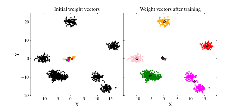
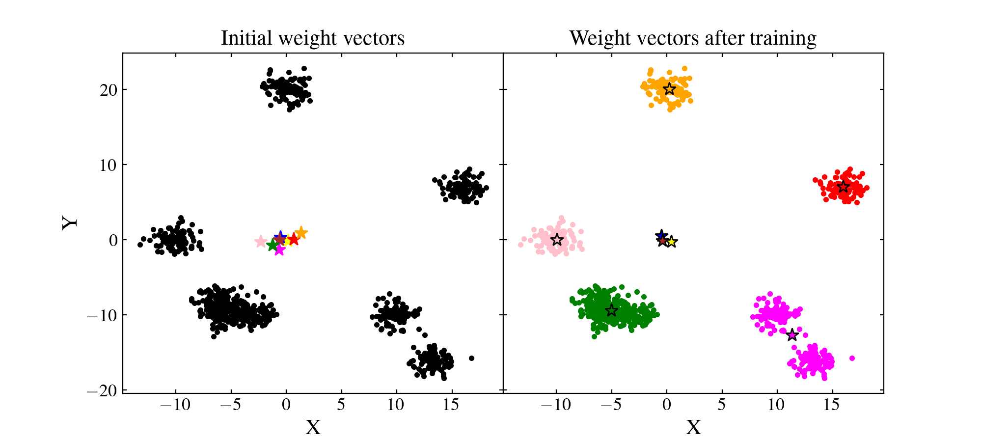
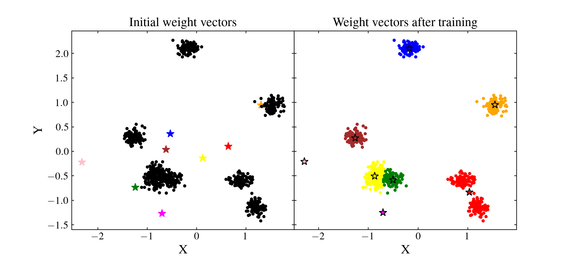
Let us see how the SOM performed. We will plot on the left figure the data with black points and the initial random weights values as coloured stars. On the right figure, we will plot the trained SOM weight values as coloured stars and the data as coloured points which matches that of their BMU:
import matplotlib.pyplot   as     plt
from   matplotlib          import rc
from   matplotlib.gridspec import GridSpec

rc('font', **{'family': 'serif', 'serif': ['Times']})
rc('text', usetex=True)

f  = plt.figure(figsize=(10, 4.5))
gs = GridSpec(1, 2, wspace=0, hspace=0)

#####################
#     Left plot     #
#####################

ax1 = f.add_subplot(gs[0])

ax1.yaxis.set_ticks_position('both')
ax1.xaxis.set_ticks_position('both')
ax1.tick_params(axis='x', which='both', direction='in', labelsize=13, length=3)
ax1.tick_params(axis='y', which='both', direction='in', labelsize=13, length=3)
ax1.set_ylabel('Y', size=16)
ax1.set_xlabel('X', size=16)
ax1.set_title('Initial weight vectors', size=16)

# We recompute the initial weight values (this is possible because we set the seed of the random generator)
rng     = np.random.default_rng(0)
weights = rng.normal(size=(2*4, nf))

colors  = ['yellow', 'r', 'b', 'orange', 'magenta', 'brown', 'pink', 'g']

# Plot neurons
for xx, yy, c in zip(weights[:, 0], weights[:, 1], colors):
   ax1.plot(xx, yy, marker='*', color=c, linestyle='none', markersize=10)

# Plot train data
ax1.plot(x, y, 'k.', linestyle='none')

######################
#     Right plot     #
######################

ax2 = f.add_subplot(gs[1])

ax2.yaxis.set_ticks_position('both')
ax2.xaxis.set_ticks_position('both')
ax2.tick_params(axis='x', which='both', direction='in', labelsize=13, length=3)
ax2.tick_params(axis='y', which='both', direction='in', labelsize=13, length=3)
ax2.set_xlabel('X', size=16)
ax2.set_title('Weight vectors after training', size=16)
ax2.set_yticklabels([])

for idx, xx, yy, c in zip(range(som.weights.shape[0]), som.weights[:, 0], som.weights[:, 1], colors):

   # Find data which have this neuron as BMU
   data_idx = data[pred == idx]

   ax2.plot(data_idx[:, 0], data_idx[:, 1], color=c, marker='.', linestyle='none')
   ax2.plot(xx, yy, marker='*', color=c, linestyle='none', markersize=10, mec='k')

plt.show()
(Source code, png, hires.png, pdf)

We see that the result if far from being optimal. Even if some clusters are recovered by the SOM, some neurons are far from where they should ideally converge. Besides, even those which are near clusters are somewhat offset from their ideal position. The reason for this effect is that the data have not been normalised. A neuron which is initialised at a privileged position with respect to some cluster will have more chance to being trained and pulled onto that cluster, making other neurons less likely to be trained efficiently.
To circumvent this problem we can normalise the data by removing the mean value and dividing by their standard deviation for each feature. This way, the majority of the data should be located in the range \([-1, 1]\), near the random initial positions of the SOM wieght vectors:
# Print mean and std before normalisation
print(f'Mean along x and y axes before normalisation: {np.nanmean(data, axis=0)}')
print(f'Standard deviation along x and y axes before normalisation: {np.nanstd(data, axis=0)}')

# Normalise each feature
new_data = (data - np.nanmean(data, axis=0))/np.nanstd(data, axis=0)

# Print mean and std after normalisation
print(f'Mean along x and y axes after normalisation: {np.nanmean(data, axis=0)}')
print(f'Standard deviation along x and y axes after normalisation: {np.nanstd(data, axis=0)}')
Results
Mean before normalisation: [ 1.70401726 -3.38087602]
Standard deviation before normalisation: [ 9.24220196 11.07705347]
Mean after normalisation: [-7.10542736e-17  0.00000000e+00]
Standard deviation after normalisation: [1. 1.]
Now, we can train again the SOM and see whether the normalisation changed anything
som    = SOM(m=2, n=4, dim=nf, lr=lr, sigma=sigma, metric=metric, max_iter=1e4, random_state=0)
som.fit(data_norm, epochs=3, shuffle=True)

# Prediction for the train dataset
pred   = som.train_bmus_

# Plotting
rc('font', **{'family': 'serif', 'serif': ['Times']})
rc('text', usetex=True)

f  = plt.figure(figsize=(10, 4.5))
gs = GridSpec(1, 2, wspace=0, hspace=0)

#####################
#     Left plot     #
#####################

ax1 = f.add_subplot(gs[0])

ax1.yaxis.set_ticks_position('both')
ax1.xaxis.set_ticks_position('both')
ax1.tick_params(axis='x', which='both', direction='in', labelsize=13, length=3)
ax1.tick_params(axis='y', which='both', direction='in', labelsize=13, length=3)
ax1.set_ylabel('Y', size=16)
ax1.set_xlabel('X', size=16)
ax1.set_title('Initial weight vectors', size=16)

# We recompute the initial weight values (this is possible because we set the seed of the random generator)
rng     = np.random.default_rng(0)
weights = rng.normal(size=(2*4, nf))

colors  = ['yellow', 'r', 'b', 'orange', 'magenta', 'brown', 'pink', 'g']

# Plot neurons
for xx, yy, c in zip(weights[:, 0], weights[:, 1], colors):
   ax1.plot(xx, yy, marker='*', color=c, linestyle='none', markersize=10)

# Plot train data
ax1.plot(data_norm[:, 0], data_norm[:, 1], 'k.', linestyle='none')

######################
#     Right plot     #
######################

ax2 = f.add_subplot(gs[1])

ax2.yaxis.set_ticks_position('both')
ax2.xaxis.set_ticks_position('both')
ax2.tick_params(axis='x', which='both', direction='in', labelsize=13, length=3)
ax2.tick_params(axis='y', which='both', direction='in', labelsize=13, length=3)
ax2.set_xlabel('X', size=16)
ax2.set_title('Weight vectors after training', size=16)
ax2.set_yticklabels([])

for idx, xx, yy, c in zip(range(som.weights.shape[0]), som.weights[:, 0], som.weights[:, 1], colors):

   # Find data which have this neuron as BMU
   data_idx = data_norm[pred == idx]

   ax2.plot(data_idx[:, 0], data_idx[:, 1], color=c, marker='.', linestyle='none')
   ax2.plot(xx, yy, marker='*', color=c, linestyle='none', markersize=10, mec='k')

plt.show()
(Source code, png, hires.png, pdf)

Important
Normalisation is not always the best option. It all comes down to the metric used.
For instance, with the chi2CigaleMetric() metric, data should not be normalised. Instead, to have an optimal SOM, one should denormalise the SOM weight vectors using unnormalise_weights=True when calling the fit() method.
See the documentation for the metric you use for more information.
Set and get extra parameters#
In the previous section we computed an additional parameter for each neuron in the SOM: the petal width. Rather than keeping such parameters in separate variables, we can integrate them into the SOM to easily access them later on.
This is done with the set() method
som.set('petal width', swidth_med)
som.set('petal width uncertainty', swidth_std)
To retrieve later on an extra parameter (e.g. petal width), then one can use the get() method
pwidth = som.get('petal width')

print('Petal width for the SOM neurons:')
print(swidth_med)
print('\nPetal width stored in the SOM:')
print(pwidth)
Results
Petal width for the SOM neurons:
[nan, nan, nan, nan, nan, nan, 3.0, 3.5, nan, 2.4, nan, 3.1, 3.8, 2.3499999999999996, 2.8, nan, nan, 2.6, 2.9, 2.75, nan, nan, 2.6500000000000004, 2.95, 3.0]

Petal width stored in the SOM:
[nan, nan, nan, nan, nan, nan, 3.0, 3.5, nan, 2.4, nan, 3.1, 3.8, 2.3499999999999996, 2.8, nan, nan, 2.6, 2.9, 2.75, nan, nan, 2.6500000000000004, 2.95, 3.0]
Save and load SOM#
A last feature of this SOM implementation is that the it can be saved at any moment and loaded back again. This is easily done using the write() method
som.write('som_save')
The SOM can be loaded back at any time later on using the read() method
newsom = SOM.read('som_save')

print('BMUs for train data:')
print(som.train_bmus_)
print('\nBMUs for train data loaded from file:')
print(newsom.train_bmus_)
Results
BMUs for train data:
[0 0 0 0 0 0 0 0 0 0 0 0 0 0 0 0 0 0 0 0 0 0 0 0 0 0 0 0 0 0 0 0 0 0 0 0 0
 0 0 0 0 0 0 0 0 0 0 0 0 0 1 0 1 0 1 0 0 0 1 0 0 0 0 0 0 0 0 0 0 0 0 0 1 0
 0 0 1 1 0 0 0 0 0 1 0 0 1 0 0 0 0 0 0 0 0 0 0 0 0 0 2 1 2 1 2 2 0 2 2 2 1
 1 2 0 1 1 1 2 2 1 2 0 2 1 2 2 1 1 1 2 2 2 1 1 1 2 1 1 0 2]

BMUs for train data loaded from file:
[0 0 0 0 0 0 0 0 0 0 0 0 0 0 0 0 0 0 0 0 0 0 0 0 0 0 0 0 0 0 0 0 0 0 0 0 0
 0 0 0 0 0 0 0 0 0 0 0 0 0 1 0 1 0 1 0 0 0 1 0 0 0 0 0 0 0 0 0 0 0 0 0 1 0
 0 0 1 1 0 0 0 0 0 1 0 0 1 0 0 0 0 0 0 0 0 0 0 0 0 0 2 1 2 1 2 2 0 2 2 2 1
 1 2 0 1 1 1 2 2 1 2 0 2 1 2 2 1 1 1 2 2 2 1 1 1 2 1 1 0 2]