Introduction#

This library provides an interface that allows to seamlessly perform resolved/pixel-per-pixel SED fitting using either Cigale or LePhare as backend. Thus, this code is not a new SED fitting package but instead relies on pre-installed SED fitting codes. It does however

significantly simplify the procedure to obtain spatially resolved maps of physical parameters (e.g. stellar mass) and
retain the full flexibility of the underlying SED fitting codes to potentially perform complex modellings.

For information on how to install the code and the SED backends, check the Setup page. The general workflow to perform resolved SED fitting with this library is as follows:

For each band, load data into a Filter object and then combine thoses objects together, along with shared information, into a single FilterList object.
Choose the SED fitting code backend.
Transform this FilterList object into a Catalogue object. This new object will be used by this library to automatically parse the input data into a catalogue with the right format for the selected SED fitting code.
Create a SED object. Each backend has its own parameters that are specific to the selected SED fitting code. This object contains the SED models and parameters used during the fit.
Run the SED fitting and recover an Output object which contains the output data, as well as methods to reconstruct the spatially resolved maps.
Plot the resulting resolved map.
Optionally, if the SED fitting was performed previously, load the output data into an Output object before plotting the results.

Tutorial#

Below we provide a step-by-step tutorial with both Cigale and LePhare as backend.

Pre-processing#

Independently of the backend used, a few assumptions are always made by the code when starting pixel-per-pixel SED fitting. Namely:

Loading data#

Creating `Filter` objects#

Whatever the backend, the first step is to load the data. To do so, two classes must be used: Filter and FilterList. First, we start by creating one Filter per band we want to fit:

import pixSED as SED

filt_435w = SED.Filter('F435W', 'data_F435W.fits', 'var_F435W.fits', 25.68, file2 = None)

Here, we consider the HST F435W band with the data stored in the file data_F435W.fits and the variance map in the file var_F435W.fits. In this example, the data are in units of $\rm e^{-}\,s^{-1}$ and the zeropoint ${\rm zpt} = 25.68$ allows to convert the data to $\rm erg\,s^{-1}\,Hz^{-1}\,cm^{-2}$ and the variance map to $\,\rm erg^2\,s^{-2}\,Hz^{-2}\,cm^{-4}$.

Note

The keyword argument file2 is optional and allows the user to provide a FITS file name that contains the data image squared. This image is used to compute the Poisson noise contribution if it is not already present in the given variance map.

To not add Poisson noise to the variance map, please use file2 = None.

Important

The input data can be given in any unit as long as the zeropoint allows to convert them to $\rm erg\,s^{-1}\,Hz^{-1}\,cm^{-2}$. The formal definition used by the code for the conversion is as follows:

\[d_{\rm conv} = d_{\rm original} \times 10^{-({\rm zpt} + 48.6) / 2.5},\]

where $d_{\rm conv}$ is the data image converted to $\rm erg\,s^{-1}\,Hz^{-1}\,cm^{-2}$, $d_{\rm original}$ is the original image given by the user, and $\rm zpt$ is the zeropoint given by the user. The same zeropoint will be used to convert the variance map.

Thus, the unit of the variance map must always be the square of the unit of the data image.

(Optional) Adding Poisson noise in quadrature#

Some error maps (or related data products such as HST weight maps) do not contain Poisson noise, in which case it should be added in quadrature. This code can handle that automatically with a few important details to keep in mind.

In practice, for Poisson noise to be added, the file2 keyword argument sould be provided to the relevant Filter objects. This keyword must be the name of a FITS file containing the input data convolved by the square of the PSF.

Note

When loading the data, the code will look for the exposure time in the FITS header keyword 'TEXPTIME'. If not found, a value of 1 will be assumed.

When the methods setCode() or genTable() are called (either automatically or by the user), it is possible to pass an extra argument to divide the value of the exposure time:

flist.genTable(texpFac=10)

In this example, the exposure time will be divided by a factor of 10 when computing the Poisson noise contribution to the total variance. If texpFac is equal to 0, no Poisson noise will be added.

Important

The user interested in adding Poisson noise to some of their variance maps is encouraged to read attentively this page.

(Optional) Recovering and updating the intermediate table#

The interested user can recover the intermediate Astropy Table as follows

table = flist.table

Furthermore, the values in this table can be updated using the genTable() method. For instance to scale up the fluxes and uncertainties by a factor 100, one can do

flist.genTable(scaleFactor=100)

Similarly, to change the bad pixel cleaning method, one can do

flist.genTable(cleanMethod=SED.misc.enum.CleanMethod.ZERO)

Note

The code automatically cleans bad pixels which are identified as having either a negative flux or a negative variance. Two cleaning methods are proposed:

pixSED.misc.enum.CleanMethod.ZERO which replaces bad pixels by a flux equal to 0 and
pixSED.misc.enum.CleanMethod.MIN which replaces bad pixels with the minimum value in the masked image.

There is also the possibility to update the SED fitting code backend as follows:

flist.setCode(SED.SEDcode.LEPHARE)

Generate a `Catalogue` object#

Because each SED fitting code expects the input data to be parsed to different formats, each code as its own Catalogue object that manages this parsing automatically. In each case, the catalogue creation is done as follows:

catalogue  = flist.toCatalogue('example')

where the first argument corresponds to the name of the output file (without extension) that will contain the catalogue used by the SED fitting code. For Cigale, this will create a CigaleCat object, whereas for LePhare this will create a LePhareCat object.

Note

For LePhare, other parameters can be given. Please refer to LePhareCat init method for further details.

Create a `SED` object#

After creating the catalogue that will contain the input data, we need to initialise the parameters of the SED fitting code along with specifying the models used for the SED fitting. Cigale and LePhare have different models and ways to handle them, so each has its own SED object to initialise:

Using Cigale as backend

Cigale works with modules that can be combined together. This includes modules such as star formation histories, single stellar populations, dust attenuation, dust emission, etc. The full list of modules that are supported by this library are listed here.

In this example, let us define a star-formation history, single stellar population, nebular emission, and dust attenuation as follows:

# Star formation history module to use
SFH        = [SED.cigmod.SFHDELAYEDBQmodule(tau_main  = [250, 500, 1000, 2000, 4000, 6000, 8000],
                                            age_main  = [2500, 5000, 7500, 10000, 12500],
                                            age_bq    = [10, 25, 50, 75, 100, 150, 200],
                                            r_sfr     = [0.0, 0.2, 0.4, 0.6, 0.8, 1.0, 1.25, 1.5, 1.75, 2.0, 5.0, 10.0],
                                            sfr_A     = [1.0],
                                            normalise = True
                                           )]

# Single Stellar population module to use
SSP        = [SED.cigmod.BC03module(imf            = SED.IMF.CHABRIER,
                                    separation_age = [8],
                                    metallicity    = [0.02]
                               )]

# Nebular emission module to use
nebular    = [SED.cigmod.NEBULARmodule(logU             = [-2.0],
                                       f_esc            = [0.0],
                                       f_dust           = [0.0],
                                       lines_width      = [300.0],
                                       include_emission = True
                                     )]

# Dust attenuation module to use
attenuation = [SED.cigmod.DUSTATT_POWERLAWmodule(Av_young           = [0.0, 0.25, 0.5, .75, 1.0, 1.25, 1.5, 1.75, 2.0, 2.25, 2.5, 2.75, 3.0],
                                                 Av_old_factor      = [0.44],
                                                 uv_bump_wavelength = [217.5],
                                                 uv_bump_width      = [35.0],
                                                 uv_bump_amplitude  = [0.0, 1.5, 3.0],
                                                 powerlaw_slope     = [-0.7],
                                                 filters            = ' & '.join(band_names)
                                                )]

Then, we can initialise the CigaleSED object as follows:

sedobj = SED.CigaleSED('example', ['F435W', 'F606W', 'F775W'],
                       uncertainties = [True]*len(band_names),
                       SFH           = SFH,
                       SSP           = SSP,
                       nebular       = nebular,
                       attenuation   = attenuation,
                      )

where 'example' is the name of the directory within which the output files will be stored, ['F435W', 'F606W', 'F775W'] is the list of filters to use for the SED fitting. The argument uncertainties can be used to define for which filters the uncertainties should be used in the fit.

Using LePhare as backend

prop = {'FILTER_LIST' : ['HST_ACS_WFC.F435W', 'HST_ACS_WFC.F606W', 'HST_ACS_WFC.F775W'],
        'ERR_SCALE'   : [0.03, 0.03, 0.03]
       }

sed  = SED.LePhareSED('example', properties=prop)

where 'example' is the name of the directory within which the output files will be stored. The keyword argument properties must be a dictionary that stores the different SED parameters for LePhare. We give a brief list of the most useful ones below:

STAR_SED [str]: stellar library list file (full path)
QSO_SED [str]: QSO list file (full path)
GAL_SED [str]: galaxy library list file (full path)
AGE_RANGE [list[float]]: minimum and maximum ages in years
FILTER_LIST [list[str]]: list of filter names used for the fit (must all be located in $LEPHAREDIR/filt directory)
Z_STEP [list[int/float]]: redshift step properties. Values are: redshift step, max redshift, redshift step for redshifts above 6 (coarser sampling).
COSMOLOGY [list[int/float]]: cosmology parameters. Values are: Hubble constant H0, baryon fraction Omegam0, cosmological constant fraction Omegalambda0.
MOD_EXTINC [list[int/float]]: minimum and maximum model extinctions
EXTINC_LAW [str]: extinction law file (in $LEPHAREDIR/ext)
EB_V [list[int/float]]: color excess E(B-V). It must contain less than 50 values.
EM_LINES [str]: whether to consider emission lines or not. Accepted values are ‘YES’ or ‘NO’.
ERR_SCALE [list[int/float]]: magnitude errors per band to add in quadrature
ERR_FACTOR [int/float]: scaling factor to apply to the errors
ZPHOTLIB [list[str]]: librairies used to compute the Chi2. Maximum number is 3.
ADD_EMLINES [str]: whether to add emission lines or not (dupplicate with EM_LINES ?). Accepted values are ‘YES’ or ‘NO’.

For the complete list of options, see LePhareOutputParam values (upper case names).

Resolved SED fitting#

Run the SED fitting#

Using Cigale as backend

Cigale can now be easily launched as follows

output = sedobj(catalogue,
                ncores              = 8,
                physical_properties = None,
                bands               = ['F435W', 'F606W', 'F775W'],
                save_best_sed       = False,
                save_chi2           = False,
                lim_flag            = False,
                blocks              = 1
               )

The first argument is the CigaleCat object created above. Then, additional keyword arguments can be passed:

ncores: number of threads to use for parallelisation
physical_properties: a list of physical property names to be computed. Providing physical_properties = None will result in all the physical properties being computed.
bands: the bands for which to estimate the fluxes in the output file
save_best_sed: whether to save the best-fit SED for each pixel being fitted
save_chi2: whether to save the chi2 for each pixel being fitted
lim_flag: whether to consider upper limits or not
blocks: number of subdivisions for the data if there are too many pixels to be fitted

This library automatically extracts output parameters and stores them into the output variable as a CigaleOutput object.

Using LePhare as backend

The LePhareSED object can be directly called to run the SED fitting. In order to avoid to load all of LePhare parameters in the output file, a list of required parameter names (see LePhareOutputParam for accepted values) must be passed as follows

params = ['MASS_INF', 'MASS_MED', 'MASS_SUP', 'SFR_INF', 'SFR_MED', 'SFR_SUP']
output = sed(catalogue, outputParams=params)

The SED fitting code then executes in the background. When running, LePhare generates various files:

file.in: Input catalogue containing data
file.para: Parameter files with all the SED fitting properties
file.output_para: List of output parameters given in the output file
file.out: Output data file

This library automatically extracts those output parameters and stores them into the output variable as a LePhareOutput object.

Important

Data given as log values in the LePhare output parameter file are converted into physical units.

For instance, MASS_MED parameter is given by LePhare by default as the decimal logarithm of the median mass in solar masses. But, in the LePhareOutput object it corresponds to the median mass in solar masses.

Before performing the SED fitting, LePhare must generate a grid of models for the stars, galaxies and QSO. These models are saved into different files located in LePhare directory, so in practice they only need to be generated once, unless one needs a new grids of models.

By default, calling the LePhareSED object always generates all of the SED models and compute their magnitudes. To disable one or more or the SED generation and/or magnitude computation, optional parameters can be passed as

params     = ['MASS_INF', 'MASS_MED', 'MASS_SUP', 'SFR_INF', 'SFR_MED', 'SFR_SUP']

skipSED    = True # Skip SED generation
skipFilter = True # Skip filters generations
skipGal    = True # Skip galaxy magnitude computation
skipQSO    = True # Skip QSO magnitude computation
skipStar   = True # Skip stellar magnitude computation

output     = sed(catalogue, outputParams=params,
                 skipSEDgen    = skipSED,
                 skipFilterGen = skipFilter,
                 skipMagQSO    = skipQSO,
                 skipMagStar   = skipStar,
                 skipMagGal    = skipGal
                )

Extract data from a previous run#

Alternatively, if the SED fitting was already run beforehand, it is possible to directly load the data without doing the fit again by directly calling CigaleOutput or LePhareOutput:

Using Cigale as backend

output = SED.CigaleOutput('example/out/results.fits')

Using Cigale as backend

output = SED.LePhareOutput('example/example.out')

Plot a resolved map#

Both CigaleOutput and LePhareOutput have a utility class that allows to reconstruct a 2D ndarray with the same shape as the input images and with the mask applied.

Using Cigale as backend

For Cigale, the only arguments that need to be passed are the parameter name to produce the resolved map for (here 'bayes.stellar.m_star') and the shape of the image:

image = output.toImage('bayes.stellar.m_star', shape=(100, 100))

Using LePhare as backend

For LePhare, more arguments are required in order to scale back the resolved map to the right unit. The first argument is the parameter name to produce the resolved map for (here 'mass_med') and then one needs to provide

the shape of the image,
the scale factor used to normalise the data (in this example 100)
the mean map used to normalise the data (which is stored in meanMap)

image = output.toImage('mass_med',
                       shape       = (100, 100),
                       scaleFactor = 100,
                       meanMap     = flist.meanMap
                      )

Note

The variable image is an Astropy Quantity. Its unit can be recovered with image.unit and its values in any unit (e.g. solar masses) as an ndarray with image.to('Msun').value

Note

Since shape, scaleFactor and meanMap are not straightforward to find, a utility method can be used to recover them automatically:

output.link(flist)
image = output.toImage('bayes.stellar.m_star')

where output is the CigaleOutput or LePhareOutput object from above and flist is the FilterList object created here.

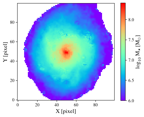
We can now generate a resolved stellar mass map:

from   matplotlib        import rc
import matplotlib        as     mpl
import matplotlib.pyplot as     plt

rc('font', **{'family': 'serif', 'serif': ['Times']})
rc('text', usetex=True)
mpl.rcParams['text.latex.preamble'] = r'\usepackage{newtxmath}'
rc('figure', figsize=(5, 4.5))

plt.imshow(np.log10(image.to('Msun').value), origin='lower', cmap='rainbow', vmin=6)
plt.xlabel('X [pixel]', size=13)
plt.ylabel('Y [pixel]', size=13)

cbar = plt.colorbar(ret, orientation='vertical', shrink=0.9)
cbar.set_label(r'$\log_{10}$ M$_{\star}$ [M$_{\odot}$]', size=13)
plt.show()

Adding Poisson noise...
Adding Poisson noise...
Adding Poisson noise...
Adding Poisson noise...
Adding Poisson noise...
Adding Poisson noise...
Adding Poisson noise...
Adding Poisson noise...
Adding Poisson noise...
Adding Poisson noise...
Adding Poisson noise...
Adding Poisson noise...
Adding Poisson noise...
Adding Poisson noise...
Adding Poisson noise...
Adding Poisson noise...
Adding Poisson noise...
Adding Poisson noise...
example/1/out/results.fits

Introduction#

Tutorial#

Pre-processing#

Loading data#

Creating Filter objects#

Combining Filter objects into a FilterList#

(Optional) Adding Poisson noise in quadrature#

(Optional) Recovering and updating the intermediate table#

Generate a Catalogue object#

Create a SED object#

Resolved SED fitting#

Run the SED fitting#

Extract data from a previous run#

Plot a resolved map#

Creating `Filter` objects#

Combining `Filter` objects into a `FilterList`#

Generate a `Catalogue` object#

Create a `SED` object#