Examples#
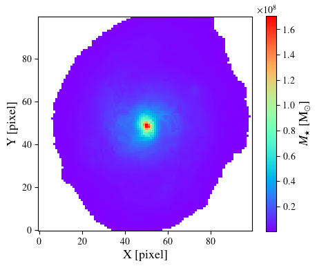
The goal of this example is to produce a resolved stellar mass map using Cigale as backend. First, we start by importing os.path module (to deal with paths independently of the OS), this library and astropy.io.fits to open the mask file.
from   astropy.io import fits
import pixSED     as     SED
import os.path    as     opath
We define the galaxy name which will be used to make a directory, the bands used for the SED fitting, their zeropoints and the absolute paths of the files containing the flux and variance maps.
Note
In this example, the variance maps do not include Poisson noise so the code will add it in quadrature. To do so, we also provide the absolute paths of the files containing the flux maps convolved with the square of the PSF.
galName    = '1'                                                                # Galaxy name
zeropoints = [25.68, 26.51, 25.69, 25.94, 24.87, 26.27, 26.23, 26.45, 25.94]    # HST zeropoints
redshift   = 0.622                                                              # Redshift of the galaxy
bands      = ['435', '606', '775', '814', '850', '105', '125', '140', '160']    # Band name used in input file names
band_names = [f'F{band}LP' if band == '850' else f'F{band}W' for band in bands] # Band names in Cigale

dataFiles  = [] # Flux maps
data2Files = [] # Flux maps convolved by the square of the PSF
varFiles   = [] # Variance maps

for band in bands:

   file    = opath.abspath(opath.join('data', f'{galName}_{band}.fits'))
   dataFiles.append(file)

   file2   = opath.abspath(opath.join('data', f'{galName}_{band}_PSF2.fits'))
   data2Files.append(file2)

   vfile   = opath.abspath(opath.join('data', f'{galName}_{band}_var.fits'))
   varFiles.append(vfile)
We also need to manually open the mask file. It must be an array of True and False values, with True for the pixels to mask.
mfile   = opath.abspath(opath.join('data', f'{galName}_mask.fits'))
with fits.open(mfile) as hdul:
   mask = hdul[0].data == 0
Then, we build the FilterList, include Poisson noise to the variance map (by passing data2 and texpFac) and we convert it to a catalogue.
Note
For Cigale, no need to normalise the data. Thus, scaleFactor will not be used and can be omitted.
filts      = []
for band, data, data2, var, zpt in zip(bands, dataFiles, data2Files, varFiles, zeropoints):
   filts.append(SED.Filter(band, data, data2, var, zpt))

flist      = SED.FilterList(filts, mask,
                            code=SED.SEDcode.LEPHARE,
                            redshift=redshift,
                            cleanMethod=SED.CleanMethod.ZERO,
                            texpFac=4,
                            #scaleFactor=1
                           )

catalogue  = flist.toCatalogue(galName)
We now have the catalogue. However, we are still missing the SED modules and parameters to start the SED fitting. Any number of modules can be given but Cigale requires at least to provide one SFHmodule and one SSPmodule. We will use the following modules:
# Star formation history module to use
SFH        = [SED.cigmod.SFHDELAYEDBQmodule(tau_main  = [250, 500, 1000, 2000, 4000, 6000, 8000],
                                            age_main  = [2500, 5000, 7500, 10000, 12500],
                                            age_bq    = [10, 25, 50, 75, 100, 150, 200],
                                            r_sfr     = [0.0, 0.2, 0.4, 0.6, 0.8, 1.0, 1.25, 1.5, 1.75, 2.0, 5.0, 10.0],
                                            sfr_A     = [1.0],
                                            normalise = True
                                           )]

# Single Stellar population module to use
SSP        = [SED.cigmod.BC03module(imf            = SED.IMF.CHABRIER,
                                    separation_age = [8],
                                    metallicity    = [0.02]
                               )]

# Nebular emission module to use
nebular    = [SED.cigmod.NEBULARmodule(logU             = [-2.0],
                                       f_esc            = [0.0],
                                       f_dust           = [0.0],
                                       lines_width      = [300.0],
                                       include_emission = True
                                     )]

# Dust attenuation module to use
attenuation = [SED.cigmod.DUSTATT_POWERLAWmodule(Av_young           = [0.0, 0.25, 0.5, .75, 1.0, 1.25, 1.5, 1.75, 2.0, 2.25, 2.5, 2.75, 3.0],
                                                 Av_old_factor      = [0.44],
                                                 uv_bump_wavelength = [217.5],
                                                 uv_bump_width      = [35.0],
                                                 uv_bump_amplitude  = [0.0, 1.5, 3.0],
                                                 powerlaw_slope     = [-0.7],
                                                 filters            = ' & '.join(band_names)
                                                )]
With all the modules stored in different variables, we can now build a CigaleSED object. This object will be used to start the SED fitting in the background and recover the output properties to reconstruct a stellar mass map.
sedobj = SED.CigaleSED(galName, band_names,
                       uncertainties = [True]*len(band_names),
                       SFH           = SFH,
                       SSP           = SSP,
                       nebular       = nebular,
                       attenuation   = attenuation,
                      )
The uncertainties argument controls for which bands the uncertainty is used during the fit. We give True for all the bands since we want to use all the uncertainties. We can now run Cigale by providing the catalogue built previously, as well as a list of extra parameters.
output = sedobj(catalogue,
                ncores              = 8,           # Number of threads to use (to be updated)
                physical_properties = None,        # None means all properties will be computed
                bands               = band_names,  # We estimate the flux for all the bands
                save_best_sed       = False,       # Whether to save in output FITS files the best sed
                save_chi2           = False,       # Whether to save the chi2 for all models
                lim_flag            = False,
                redshift_decimals   = 2,
                blocks              = 1
               )
Once the fit is complete, we can plot the stellar mass map. To do so, we can use the output variable (of type CigaleOutput).
Note
For Cigale, we must provide only the shape of the map we want to reconstruct. This can be done either when using the toImage() method or by linking the original FilterList object to the output variable using the link() method.
from   matplotlib        import rc
import matplotlib        as     mpl
import matplotlib.pyplot as     plt

output.link(flist)
mass_star = output.toImage('best.stellar.m_star')

rc('font', **{'family': 'serif', 'serif': ['Times']})
rc('text', usetex=True)
mpl.rcParams['text.latex.preamble'] = r'\usepackage{newtxmath}'
rc('figure', figsize=(5, 4.5))

ret = plt.imshow(mass_star.data, origin='lower', cmap='rainbow')
plt.xlabel('X [pixel]', size=13)
plt.ylabel('Y [pixel]', size=13)

cbar = plt.colorbar(ret, orientation='vertical', shrink=0.9)
cbar.set_label(r'$M_{\star}$ [M$_{\odot}$]', size=13)
plt.show()
Adding Poisson noise...
Adding Poisson noise...
Adding Poisson noise...
Adding Poisson noise...
Adding Poisson noise...
Adding Poisson noise...
Adding Poisson noise...
Adding Poisson noise...
Adding Poisson noise...
example/1/out/results.fits

In this example, we want to generate a resolved stellar mass map using LePhare. We start by importing os.path module (to deal with paths independently of the OS), this library and astropy.io.fits to open the mask file.
from   astropy.io import fits
import os.path    as     opath
import pixSED     as     SED
We define the galaxy name, the bands used, their zeropoints and the absolute path of the flux and variance maps.
Note
In this example, the variance maps do not include Poisson noise so the code will add it in quadrature. To do so, we also provide the absolute paths of the files containing the flux maps convolved with the square of the PSF.
# Define data file names
galName    = '1'                                                             # Galaxy number
zeropoints = [25.68, 26.51, 25.69, 25.94, 24.87, 26.27, 26.23, 26.45, 25.94] # HST zeropoints
redshift   = 0.622                                                           # Redshift of the galaxy
bands      = ['435', '606', '775', '814', '850', '105', '125', '140', '160'] # Bands
band_names = ['ACS_WFC.F435W', 'ACS_WFC.F606W', 'ACS_WFC.F775W',             # Names of the band for LePhare
              'ACS_WFC.F814W', 'ACS_WFC.F850LP', 'WFC3_IR.F105W',
              'WFC3_IR.F125W', 'WFC3_IR.F140W', 'WFC3_IR.F160W']

dataFiles  = [] # Flux maps
data2Files = [] # Flux maps convolved by the PSF squared
varFiles   = [] # Variance maps

for band in bands:

   file    = opath.abspath(opath.join('data', f'{galName}_{band}.fits'))
   dataFiles.append(file)

   file2   = opath.abspath(opath.join('data', f'{galName}_{band}_PSF2.fits'))
   data2Files.append(file2)

   vfile   = opath.abspath(opath.join('data', f'{galName}_{band}_var.fits'))
   varFiles.append(vfile)
We also need to manually open the mask file. It must be an array of True and False values, with True for pixels to be masked.
mfile      = opath.abspath(opath.join('data', f'{galName}_mask.fits'))
with fits.open(mfile) as hdul:
   mask    = hdul[0].data == 0
Then, we build the filter list, update the table to include Poisson noise to the variance map and convert it to a catalogue
filts      = []
for band, data, data2, var, zpt in zip(bands, dataFiles, data2Files, varFiles, zeropoints):
   filts.append(SED.Filter(band, data, data2, var, zpt))

flist      = SED.FilterList(filts, mask, code=SED.SEDcode.LEPHARE, redshift=redshift)
flist.genTable(cleanMethod=SED.CleanMethod.ZERO, scaleFactor=100, texpFac=4)
catalogue  = flist.toCatalogue(f'{galName}')
We also need to make a sed object. To do so, we provide a few parameters, namely the filters file names (relative to $LEPHAREDIR/filt directory) and the quadratic errors added to each filter
hst_filt   = [] # Filter names for LePhare
err        = [] # Quadratic errors to add to the magnitudes of each band

for band in band_names:
   filt    = opath.join('hst_perso', f'HST_{band}')
   hst_filt.append(filt)
   err.append(0.03)

properties = {'FILTER_LIST' : hst_filt, 'ERR_SCALE' : err}
sed        = SED.LePhareSED(galName, properties=properties)
We can now run LePhare linking the data catalogue and providing a list of parameters to extract from the SED fitting
params     = ['MASS_BEST', 'MASS_INF', 'MASS_MED', 'MASS_SUP', 'SFR_BEST', 'SFR_INF', 'SFR_MED', 'SFR_SUP']
skip       = {'skipSEDgen' : True, 'skipFilterGen' : True, 'skipMagGal' : True, 'skipMagQSO' : True, 'skipMagStar' : True}
output     = sed(catalogue, outputParams=params, **skip)
To generate a resolved stellar mass map we need to provide additional parameters. The simplest method is to link the filter list to the output object
from   matplotlib        import rc
import matplotlib        as     mpl
import matplotlib.pyplot as     plt

output.link(flist)
mass_star = output.toImage('mass_med')

rc('font', **{'family': 'serif', 'serif': ['Times']})
rc('text', usetex=True)
mpl.rcParams['text.latex.preamble'] = r'\usepackage{newtxmath}'
rc('figure', figsize=(5, 4.5))

ret = plt.imshow(mass_star.data, origin='lower', cmap='rainbow')
plt.xlabel('X [pixel]', size=13)
plt.ylabel('Y [pixel]', size=13)

cbar = plt.colorbar(ret, orientation='vertical', shrink=0.9)
cbar.set_label(r'$M_{\star}$ [M$_{\odot}$]', size=13)
plt.show()
Adding Poisson noise...
Adding Poisson noise...
Adding Poisson noise...
Adding Poisson noise...
Adding Poisson noise...
Adding Poisson noise...
Adding Poisson noise...
Adding Poisson noise...
Adding Poisson noise...
Adding Poisson noise...
Adding Poisson noise...
Adding Poisson noise...
Adding Poisson noise...
Adding Poisson noise...
Adding Poisson noise...
Adding Poisson noise...
Adding Poisson noise...
Adding Poisson noise...

This example follows from the previous one. Thus, it is assumed that the SED fitting has already been performed with LePhare and that there is an associated output file named example/1/1.out.
Because fluxes had to be scaled up in order to be processed by LePhare, we will need the mean map, scale factor and exposure time in order to scale back the extensive output properties (including mass and SFR). First, we must start by building the FilterList oject:
from   astropy.io import fits
import os.path    as     opath
import pixSED     as     SED

galName    = '1'
zeropoints = [25.68, 26.51, 25.69, 25.94, 24.87, 26.27, 26.23, 26.45, 25.94]
redshift   = 0.622
bands      = ['435', '606', '775', '814', '850', '105', '125', '140', '160']

dataFiles  = []
data2Files = [] # flux maps convolved by the square of the PSF
varFiles   = []

for band in bands:

   file    = opath.abspath(opath.join('data', f'{galName}_{band}.fits'))
   dataFiles.append(file)

   file2   = opath.abspath(opath.join('data', f'{galName}_{band}_PSF2.fits'))
   data2Files.append(file2)

   vfile   = opath.abspath(opath.join('data', f'{galName}_{band}_var.fits'))
   varFiles.append(vfile)

mfile      = opath.abspath(opath.join('data', f'{galName}_mask.fits'))
with fits.open(mfile) as hdul:
   mask    = hdul[0].data == 0

filts      = []
for band, data, data2, var, zpt in zip(bands, dataFiles, data2Files, varFiles, zeropoints):
   filts.append(sed.Filter(band, file, file2, var, zpt))

flist      = SED.FilterList(filts, mask, code=SED.SEDcode.LEPHARE, redshift=redshift)
flist.genTable(cleanMethod=SED.CleanMethod.ZERO, scaleFactor=100, texpFac=4)
This FilterList object now contains all the information required to scale back the data to the right unit. So, we just have to recover the output from LePhare and link the FilterList to this object.
output = sed.LePhareOutput('1/1.out')
output.link(flist)
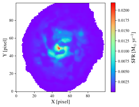
We can now generate a resolved map for the median SFR
from   matplotlib        import rc
import matplotlib        as     mpl
import matplotlib.pyplot as     plt

rc('font', **{'family': 'serif', 'serif': ['Times']})
rc('text', usetex=True)
mpl.rcParams['text.latex.preamble'] = r'\usepackage{newtxmath}'
rc('figure', figsize=(5, 4.5))

sfr = output.toImage('sfr_med')

plt.imshow(sfr.data, origin='lower', cmap='rainbow')
plt.xlabel('X [pixel]', size=13)
plt.ylabel('Y [pixel]', size=13)

cbar = plt.colorbar(ret, orientation='vertical', shrink=0.9)
cbar.set_label(r'SFR [M$_{\odot}$ yr$^{-1}$]', size=13)
plt.show()
Adding Poisson noise...
Adding Poisson noise...
Adding Poisson noise...
Adding Poisson noise...
Adding Poisson noise...
Adding Poisson noise...
Adding Poisson noise...
Adding Poisson noise...
Adding Poisson noise...
Adding Poisson noise...
Adding Poisson noise...
Adding Poisson noise...
Adding Poisson noise...
Adding Poisson noise...
Adding Poisson noise...
Adding Poisson noise...
Adding Poisson noise...
Adding Poisson noise...
