Installation and dependencies

This software was developped with python version 3.10 and the following dependencies: numpy (v2.0.1), astropy (v6.1.7), regions (v0.10), matplotlib (v3.10.0). It can be installed with the following command

$ conda env create -f environment.yml

Then, activate the conda environment to start using it. If you plan to run the provided examples, also consider installing marimo with

$ pip install marimo

General description

This is the documentation page for the ‘clump finder’ algorithm used in Mercier et al. (2025). The code used in the paper can be found in the associated repository.

The goal of the algorithm is to find contiguous structures of pixels in an image given that:

1. each pixel is brighther than a given threshold and

2. the contiguous structure is more extended than a given area.

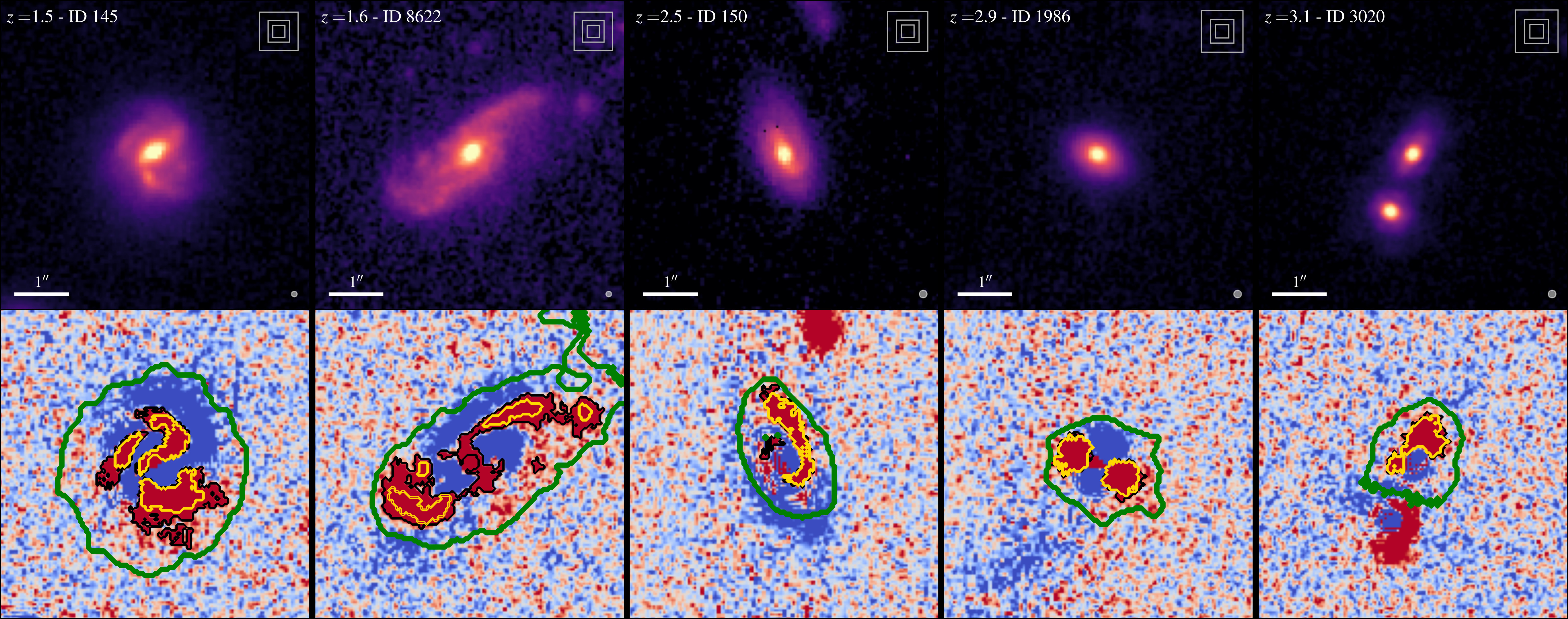
Examples of substructure detections.

This algorithm can be used to detect substructures in residual images as follows

from finder import ClumpFinder

cf = ClumpFinder(
    image, mask, mask_bg, mask_bulge
)

cf.detect(model, flux_threshold, surface_threshold)

where image is the cutout of the galaxy, model is its 2D model (i.e. image - model are the residuals), mask is a boolean array selecting pixels associated to the galaxy, mask_bg is a boolean array selecting pixels associated to background-dominated regions, mask_bulge is an optional boolean array used to select and mask pixels within the central bulge, flux_threshold is the flux threshold applied at the pixel level, and surface_threshold is the surface threshold used to select contiguous substructures.

Modes of detection

Two modes of detection were used in the paper:

1. An optimal detection whereby all substructures above user-defined flux and surface thresholds are detected.

2. An intrinsic detection whereby the detection thresholds are varied as a function of redshift to allow the detection of substructures down to similar levels of physical area and intrinsic luminosity.

Optimal detection

In Mercier et al. (2025), the optimal detection is carried out using a fixed surface threshold of \(20\,\rm pixels\) and a \(2\sigma\) flux threshold, where \(\sigma\) is the standard deviation of the background pixels located around the galaxy.

We provide a function called bg_threshold_n_sigma() that calculates \(n \sigma\) and that can be used to estimate the flux threshold for a given galaxy as follows

from finder import bg_threshold_n_sigma

two_sigma = bg_threshold_n_sigma(
    image, model, mask_bg,
    n_sigma = 2
)

If image corresponds to the residuals, then one can pass model = 0. Instead, if one is interested in estimating the lowest flux threshold required to not detect any substructure in the background dominated regions around the galaxy (i.e. the optimal threshold), one can use the find_bg_threshold() as follows

from finder import find_bg_threshold

lowest = find_bg_threshold(
    image, model, mask_bg, 20,
    positive  = True
    precision = 0.1
)

Note that using find_bg_threshold() requires defining a surface detection threshold. Furthermore, the value may differ depending on whether one is interested in positive (over-densities in residuals) or negative (under-densities) substructures. Finally, this optimal threshold is found by dichotomy which stops after a given precision is reached. This precision may need to be adjusted based on the units of the image.

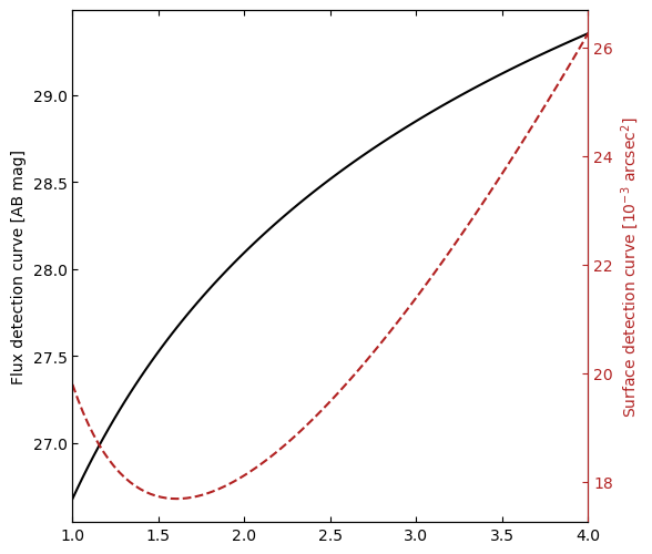
Intrinsic detection

The second detection method used in Mercier et al. (2025) is the intrinsic one. This method has already been calibrated for the sample used in the paper and we provide the functions flux_detection_curve_pixel_level() and surface_detection_curve() to readily get the detection criteria used in the paper as a function of redshift. We also provide the mag_detection_curve() function to estimate the magnitude of the faintest detectable substructure at a given redshift.

For instance, to reproduce Fig.B.3, one can use the following code:

from   finder import mag_detection_curve, surface_detection_curve
import matplotlib.pyplot as plt
import astropy.cosmology as cosmology
import numpy as np

cosmo = cosmology.FlatLambdaCDM(70, 0.3)
z     = np.linspace(1, 4, 100)

scrit = surface_detection_curve(z, cosmo)
mcrit = mag_detection_curve(z, cosmo)

f  = plt.figure(figsize=(6, 6))
ax = f.add_subplot(111)
ax.tick_params(direction='in', top=True)

plt.plot(z, mcrit, color='k')
plt.ylabel('Flux detection curve [AB mag]')

# Showing surface criterion in 1e-3 arcsec^2
ax2 = ax.twinx()
ax2.tick_params(direction='in', right=True, left=False, color='firebrick', labelcolor='firebrick')
ax2.spines['right'].set_color('firebrick')

plt.plot(z, scrit * 1e3, color='firebrick', ls='--')
plt.ylabel('Surface detection curve [$10^{-3}$ arcsec$^2$]', color='firebrick')
plt.xlabel('Redshift')

plt.xlim(1, 4)
plt.show()